 (A
larger size version of this picture may also be viewed.)
(A
larger size version of this picture may also be viewed.)
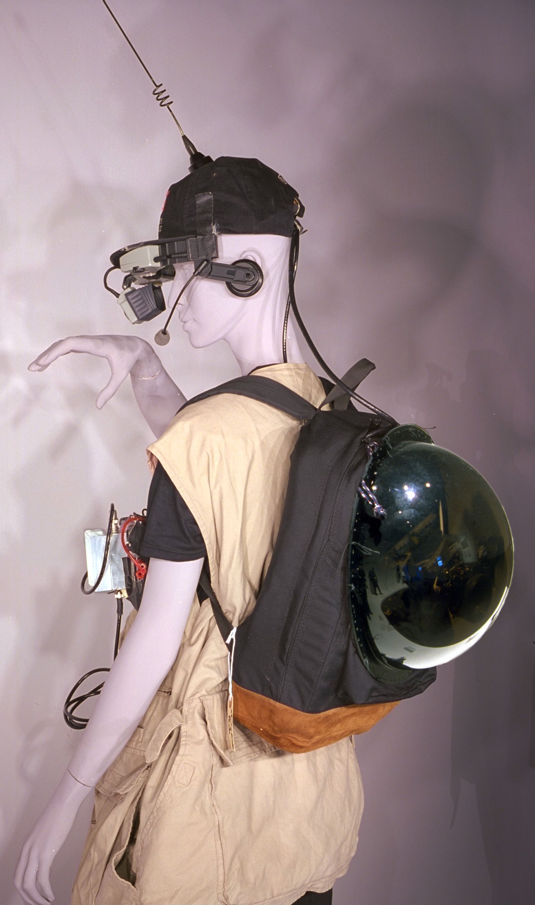
A general description of radomes may be found in http://www.radome.net/ although the emphasis has traditionally been on radomes the size of a large building rather than in sizes meant to be worn for a battery operated portable system.
This approach to Fourier analysis is called "Time Frequency" (TF) analysis, which will form the basis of this lab.
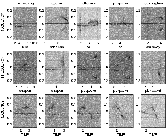
Unlike video camera systems, radar provides a much richer information space, where a single "pixel" in the radar image actually shows a lot of information, such as Doppler and range. For example, the radar can provide a "snapshot" of whether or not objects are moving toward or away from the radar, and how fast, whereas we cannot tell by looking at an ordinary photograph whether objects are moving toward or away from us. Even in video, we only see that objects are getting larger in our field of view to see that they are getting closer, but we don't get this information directly. In radar vision systems we get Doppler information directly.
The radar used in this lab transmits at approximately 24 gigahertz, so that if objects are not moving relative to the radar, the return signal is 24 gigahertz. However, if moving toward the radar, the return is slightly higher, and if moving away, slightly lower. By sampling out the transmitted frequency of 24 gigahertz, we obtain a signal that contains positive frequencies for objects coming toward the radar, and negative if going away.
Some sketches of examples of Doppler information from various situations
appear below:
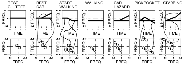
Fig. CAPTION:
REST CLUTTER: radar return when the author (wearing the radar)
is standing still;
REST CAR: a stopped car is set in motion by stepping on the accelerator,
so that a roughly constant force of the engine is exerted against the
constant mass of the car, while the author (wearing the radar) is standing
still.
START WALKING: The author stands still for one second, and then decides to
start walking. The decision to start walking is instantaneous, but the human
body applies a roughly constant degree of force to its constant mass, causing
it to accelerate until it reaches the desired walking speed, which takes
approximately 1 second. Finally the author walks at this speed for another
one second. All of the clutter behind the author (e.g. the ground, buildings,
lamp posts, etc.) is moving away from the author, so it moves into negative
frequencies.
WALKING: at a constant pace, all of the clutter has a constant (negative)
frequency. CAR HAZARD: while the author is walking forward, a parked car
is switched into gear at time 1 second. It accelerates toward the author.
The system detects this situation as a possible hazard, and brings an
image up on the screen. PICKPOCKET: rare but unique radar signature
of a person lunging up behind the author and then suddenly switching to
a decelerating mode (at time 1 second), causing reduction in velocity
to match that of the author (at time 2 seconds) followed by a retreat
away from the author.
STABBING: acceleration of attacker's body toward author, followed by
a swing of the arm (initiated at time 2 seconds) toward the author.
Below each set of time varying frequency spectra there is shown the chirplet transform. Ignore this unless you're aiming for the optional bonus question.
A typical example of a radar data test set, comprising half a second
(4000 points) of radar data starting from t=1.5 seconds and running to
t=2 seconds is shown in the following figure:
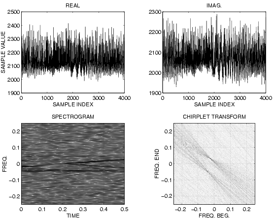
CAPTION: Most radar systems do not provide separate real and imaginary
components and therefore cannot distinguish between postive and negative
frequencies (e.g. whether an object is moving toward the radar or going
away from it). The author's radar system provides in-phase and
quadrature components:
REAL and IMAGinary plots for 4000 points (half a second) of radar data
are shown. The author was walking at a brisk pace, while a car was
accelerating toward the author.
From the Time Frequency distribution of this data, we can
see the ground clutter moving away and the car accelerating toward the
author. The Chirplet Transform shows two distinct peaks, one
corresponding to all of the ground clutter (which is all moving away
at the same speed) and the other corresponding to the accelerating car.
The radar is a crude home brew system, with interface to an
Industry Standards Association (ISA) bus, and no appreciable
effort at ensuring proper calibration was expended.
Thus there is a good deal of distortion, such as mirroring in the
FREQ=0 axis, as shown in the following Figure:
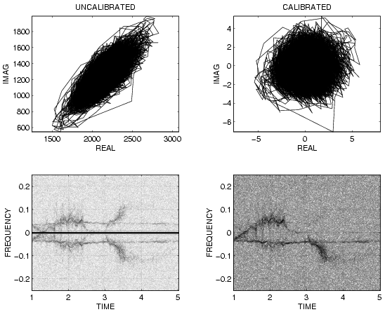
CAPTION: The author's homebrew radar generates a great deal of distortion.
Notice, for example, that a plot of real versus imaginary data shows a strong
correlation between real and imaginary axes, as well as an unequal
gain in the real and imaginary axes respectively (note also the unequal signal
strength of REAL and IMAG returns in the previous figure as well).
Note also the DC offset which gives rise to a strong signal at f=0,
even though there was nothing moving at exactly the same speed as the author
(e.g. nothing that could have given rise to a strong signal at f=0).
Rather than trying to calibrate the radar exactly,
and to remove DC offset in the circuits (all circuits were
DC coupled), and risk losing low frequency components,
these problems were mitigated by applying a calibration program to the
data. This procedure subtracted the DC offset inherent in the system,
and computed the inverse of the complex Choleski factorization of the covariance
matrix (e.g. covz defined as covariance of real and imaginary parts), which was
then applied to the data. Notice how the CALIBRATED data forms an
approximately isotropic circular blob centered at the origin when plotted as
REAL versus IMAGinary. Notice also the removal of the mirroring in the
FREQ=0 axis in the CALIBRATED data, which was quite strong in the
UNCALIBRATED data.